Calibration Pipeline
TL;DR;
We provide a geometric camera calibration pipeline using monitors as active targets, with one target for all camera types. It delivers highly consistent, repeatable, and reproducible results with up to 10 µm decoding uncertainty. Supports common OpenCV camera models and our custom free-form model, suitable for any optics. Easy integration via Docker or C++ library. It runs on CPU or CUDA / Metal GPU, on-device or server-side.
Monitor as calibration target
An obvious way to use a monitor as a calibration target is to display arbitrary patterns on it: ChArUco boards, checkerboards, circle grids, or any other custom designs. The same screen can present different target types, scaled to any desired size, while maintaining full control over the geometry and behavior of the calibration pattern. In principle, a dynamic display could replace many static calibration targets.
Why has this not become the standard approach? In fact, to a large extent, it already has. The manufacturing quality of modern monitors is sufficiently high for many applications: pixel geometry is stable and well-defined, and screen flatness is adequate for precise work. In practical scenarios, the achievable decoding uncertainty can reach the level of a few tens of microns (see our experiment)
Another potential concern when using a monitor is the moiré effect. The camera may partially resolve the subpixel structure or the black grid between display pixels, which can interfere with pattern decoding. This issue can be effectively mitigated by acquiring images with slight defocus. In this regime, the calibration pattern remains clearly visible, while the high-frequency pixel structure, and thus the moiré artifacts, are blurred out.
Therefore, using a monitor as a calibration target is not only feasible but fully legitimate for a wide range of precision calibration tasks.
Method of active targets (MAT)
We have already discussed that a camera can be calibrated using well-known static patterns such as checkerboards. However, when using a monitor as a target, we have full control over what is displayed. This allows us to exploit the dynamic nature of the screen and extract significantly more information than is possible with static patterns.
Static patterns suffer from several inherent limitations:
- Focus requirement. The pattern must be sharply in focus (or very close to it). Otherwise, feature localization degrades. At the same time, if the camera is too well focused on the pixel grid, moiré effects may appear due to interference between the sensor and display pixel structures.
- Discrete pixel structure. The geometry of printed or displayed reference points (e.g., checkerboard corners) is tied to the monitor’s pixel grid. The finite pixel size and the dark gaps between pixels introduce bias and increase decoding uncertainty.
- Border losses. Reference points near the screen boundaries are often partially visible or distorted and are therefore ignored by detection algorithms, leading to systematic undersampling near the edges.
- Dependence on the monitor pixel size. When using discrete features (e.g., checkerboard corners), the achievable localization precision is fundamentally limited by the monitor pixel pitch and the contrast structure of individual pixels. Even with subpixel refinement, the monitor pixel size influences the lower bound of achievable uncertainty.
Can these limitations be overcome? Yes. A solution has been proposed in optical metrology, a recent description can be found in [1]. The structured illumination demonstrates a fundamentally different approach: instead of detecting discrete feature points, the screen displays a sequence of phase-shifted cosine patterns.

Why this improves quality
1. No discrete reference points
There are no isolated “features” whose geometry depends on pixel edges. Instead, the entire screen contributes information. Every pixel is encoded continuously and uniformly.
2. Subpixel precision beyond display pixel pitch
Although the display is discrete, phase estimation is an intensity-based measurement. The phase can be estimated with precision far below one display pixel, limited primarily by:
- signal-to-noise ratio
- camera noise
- optical blur
This removes the hard dependency on monitor pixel size that static patterns suffer from.
3. No border exclusion
Since encoding is continuous over the entire visible area, usable data extend up to the edges of the screen (except for minimal margin due to filtering or visibility limits).
4. Reduced bias from pixel structure
Because phase is extracted from multiple frames and averaged over spatial neighborhoods, high-frequency artifacts such as the display’s subpixel grid or small intensity inhomogeneities are largely suppressed.
5. Quantifiable uncertainty
The phase noise can be analytically predicted from intensity noise (as shown in the cited work). This allows one to estimate decoding uncertainty per pixel, which is extremely valuable for metrological calibration.
6. Focus becomes less critical
Slight defocus can actually be beneficial: it suppresses moiré artifacts caused by interference between the display pixel grid and the camera sensor, while the smooth cosine patterns remain robust under moderate blur. In contrast, checkerboard corners and other sharp geometric features degrade rapidly when the image is even slightly out of focus, leading to reduced localization accuracy.
This provides a practical advantage when calibrating cameras designed for long working distances. With phase-shifted cosine patterns, the camera does not need to be perfectly focused on the calibration target. In fact, it can be intentionally defocused to suppress pixel-grid artifacts without compromising decoding precision.
As a result, calibration can be performed at significantly shorter distances than the nominal focus distance of the lens. In one of our experiments, we successfully calibrated a camera configured for a 10-meter focus distance while collecting calibration data at only 1.5 meters. Despite the strong defocus, the resulting calibration quality remained high.
ML-inspired calibration approach
We treat camera calibration as a machine learning problem: the camera model is “trained” to achieve optimal performance on a given dataset.
The calibration workflow follows principles commonly used in machine learning. Model fitting and evaluation are performed on separate datasets, and the model complexity is chosen to avoid both underfitting and overfitting. Depending on the application requirements, we can employ either classical parametric models (such as those implemented in OpenCV) or more flexible models like our free-form model capable of describing complex optical systems
To assess calibration quality, we use metrology-oriented metrics that go beyond simple agreement between the model and the calibration data. In particular, we evaluate:
- Consistency - how well the calibrated model explains the calibration data;
- Reproducibility - how stable the results remain if the calibration is repeated with independently collected data;
- Reliability - the expected measurement uncertainty when the calibrated model is used in real application scenarios.
These metrics correspond naturally to concepts from machine learning such as training loss, generalization ability, and uncertainty estimation.
Model validation is performed using K-fold cross-validation. The collected poses are divided into several subsets, and multiple calibrations are performed using different training/testing splits. For stable model classes (such as our free-form models), the resulting models can be averaged to obtain a robust final estimate. For less stable parametric models (such as OpenCV models), we select the calibration instance that demonstrates the best validation performance.
Novel Quality Metrics
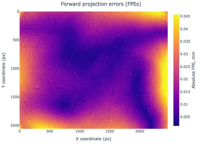
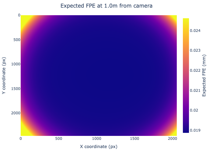
In addition to classical validation metrics such as reprojection error (RPE) and RMS error, we employ two complementary measures: forward projection error (FPE) and expected forward projection error (EFPE).
Both metrics can be used to compare different cameras against each other when selecting a camera that best suits a given application scenario. Since FPE and expected FPE are expressed in physical units in the 3D world rather than in pixels, they provide a direct estimate of how accurately the calibrated camera model predicts the positions of view rays in space. This makes it possible to evaluate and compare the geometric performance of different cameras, lenses, or calibration models in terms that are directly relevant for real-world measurements.
For example, expected FPE maps describe the uncertainty of view ray localization induced by uncertainties in the calibrated model parameters. These values can be propagated to any working distance and therefore allow estimating the expected geometric errors in a specific application setup. As a result, cameras can be compared objectively by evaluating their predicted 3D measurement accuracy within the intended field of view and working distance.
FPE evaluates the discrepancy directly in the 3D world by comparing the decoded target coordinates with the intersection of the predicted view rays and the calibration plane. Unlike pixel-based RPE, FPE is expressed in physical units (e.g., millimeters, micrometers), making it directly interpretable for metrological applications.
EFPE, in turn, quantifies the expected forward projection error induced by uncertainties in the calibrated model parameters. It translates the covariance matrix for intrinsic model parameters into predicted 3D localization uncertainty on a pre-defined surface, providing a physically meaningful measure of the model’s reliability in downstream measurements.
Together, these metrics allow us not only to assess consistency with calibration data, but also to estimate the expected real-world performance of the calibrated camera model.
More Stability and Accuracy with a Free-Form Model
For maximum performance, we have developed an advanced multi-parametric free-form calibration model. This model is capable of capturing subtle optical effects and fine-scale geometric deviations that cannot be represented by classical parametric models (such as “pinhole + several polynomial distortions”).
As a result, error levels become significantly more uniform across the entire sensor area — reducing the typical discrepancy between the image center and the corners. The model provides consistent error behavior over the full field of view, which is especially important in high-precision metrological applications.
From a data perspective, the model can be interpreted as a dense mapping (effectively a structured lookup table) that assigns a calibrated 3D view ray to every camera pixel. It is optics-agnostic; in particular, some versions support non-central projection geometries. This means it can accurately represent multi-element optics, tilted sensor systems, or complex lens assemblies without a single effective pinhole.
Due to its flexibility and dimensionality, this model is not directly compatible with standard frameworks such as OpenCV or MATLAB, which rely on compact parametric representations. Therefore, we provide dedicated libraries and tools to work with this model, including efficient routines for ray evaluation, image undistortion, reprojection, and integration into downstream vision or metrology pipelines.
Example of our Calibration
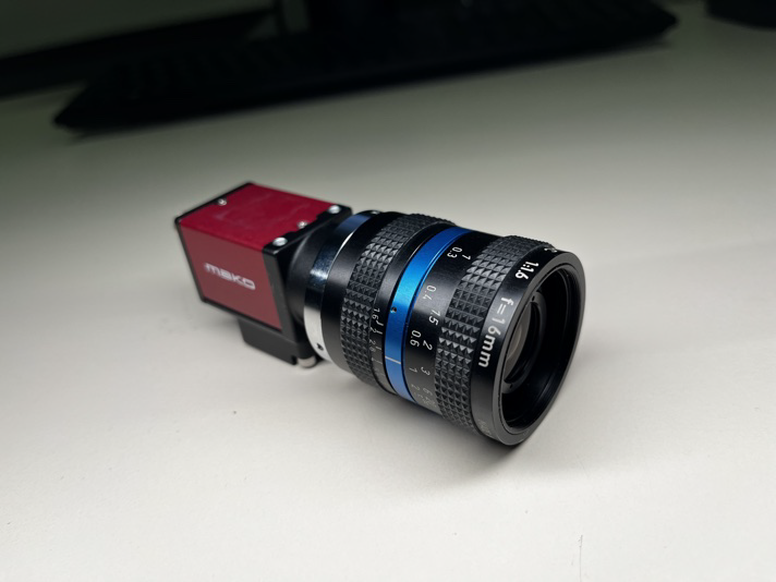
To check the best possible calibration results, we have calibrated in our experiment a 5MP industrial camera MAKO G-507 B from Allied Vision Technologies. It has a monochromatic CMOS sensor with the diagonal of 11.1 mm, the resolution of 2464 x 2056 pixels (i.e., the pixel pitch is 3.45 μm x 3.45 μm), and records data with 12-bit image bit depth. The camera is coupled with a 16 mm LINOS MeVis-C lens.
During the calibration we have collected data from 34 camera positions. At each position, the camera remained static, while the screen looped through a sequence of coded patterns: ChArUco and MAT.
| Scenario | Data Source | Reference Points | Point Noise (µm) | Camera Model | RMS RPE (px) | RMS FPE (µm) | Key Result |
|---|---|---|---|---|---|---|---|
| Scenario I (Baseline) | ChArUco | 6364 | ~130 µm | OpenCV standard model | 0.68 | 85 | High-quality standard calibration |
| Scenario II | MAT (subsampled) | ~8M | ~17 ± 10 µm | OpenCV standard model | 0.23 | 33 | Much more stable calibration, no outlier regions |
| Scenario III | MAT | ~8M | ~17 ± 10 µm | Free-form model | 0.21 | 28 | Extremely uniform model-to-data agreement |
Key Improvements
| Transition | RPE Improvement | FPE Improvement | Main Reason |
|---|---|---|---|
| Scenario I → II | ~3× lower | ~2.6× lower | Much more precise target measurements (MAT vs CharUCO) |
| Scenario II → III | Slight improvement | Slight improvement | More flexible camera model |
Measurement Quality of Targets
| Target Type | Estimated Noise |
|---|---|
| CharUCO corners | ~130 µm |
| MAT decoded positions | ~17 ± 10 µm |
| MAT decoding limit (design goal) | ~10 µm |
There are two main takeaways: the largest improvements in RPE/FPE comes from better measurement data using active targets and the free-form camera model mainly improves stability and uniformity of the calibration rather than dramatically reducing global metrics.
Calibration Speed
Speed of the calibration is the second key parameter we focus on, alongside calibration quality.
Depending on the application requirements, calibration may involve one or multiple poses, with multiple frames acquired per pose. The computational part of the calibration pipeline itself is highly efficient and runs comfortably even on modest GPUs. In ideal conditions, the overall calibration runtime can approach the time needed for data acquisition.
In practice, however, total system performance is influenced by additional factors, such as:
- The monitor’s switching time between displayed patterns
- Camera exposure time and frame rate
- Data transfer bandwidth between camera and processing system
To achieve optimal performance, we apply several strategies:
- Single-pose calibration approach. In some scenarios, calibration can be performed from a single pose (this may require additional hardware components or controlled setup adjustments).
- Reducing frames per pose. The number of phase-shifted frames can be adjusted depending on the required accuracy level.
- Controlled environment. Stabilizing illumination, mechanical setup, and focus reduces noise and allows fewer frames per pose without sacrificing quality.
- Multi-camera calibration. Multiple cameras can be calibrated simultaneously using the same monitor, significantly increasing throughput in production environments.
To provide reliable estimates of achievable performance for a specific setup, we simulate the entire calibration process. This allows us to predict acquisition time, computational load, bottlenecks, and scalability before deployment.
Integration
In its simplest form, the calibration pipeline is delivered as a standalone software component (C++), accessible via an API. It runs on CPU or GPU (CUDA for NVIDIA, Metal for Apple platforms) and uses a standard flat monitor as the active calibration target.
For more advanced scenarios, the system can be deployed as a server-side solution (with Docker support), running on multi-GPU infrastructure for high-throughput environments. Hardware setups may include large-format displays (e.g., 85-inch panels) mechanically reinforced with aluminum frames to ensure geometric stability or use a micro-LED or IPad screen. The pipeline can also be adapted for FPGA implementations when maximum speed is required, or deployed directly on devices: for example, enabling on-device self-calibration in fleets of smartphones or distributed camera systems.
The core principle is flexibility: there is no single fixed configuration of the calibration pipeline. Its final architecture is tailored to the specific task, performance requirements, and available hardware. Our solution is modular and adaptable, ensuring an optimal balance between accuracy, speed, scalability, and integration constraints.
Simulation
To answer practical questions such as how the final solution will look, what level of accuracy can be expected, how the hardware and integration should be designed, and what performance can be achieved, one of our key steps is simulation.
We simulate the entire calibration pipeline using physically-accurate rendering tools such as Mitsuba. In these simulations, we model the specific cameras under consideration, generate synthetic calibration data under realistic conditions (including optics, noise, blur, and geometry), and then run the full calibration procedure on the simulated data.
This allows us to:
- Predict achievable accuracy before hardware deployment
- Evaluate robustness under realistic noise and environmental conditions
- Compare different camera models and calibration strategies
- Optimize the calibration setup (display size, distances, number of poses, pattern parameters)
- Estimate computational performance and scalability
By performing this end-to-end virtual validation, we can adjust the calibration design in advance and significantly reduce risks, integration time, and unexpected performance limitations in the real system.

For advanced scenarios, we can also provide high-fidelity visual simulations built in Unreal Engine. These simulations allow us to present realistic, interactive environments that clearly demonstrate the calibration workflow, system behavior, and expected performance, particularly useful when communicating with stakeholders or decision-makers.
While our physics-based simulations focus on quantitative accuracy and validation, Unreal Engine visualizations provide an intuitive and visually compelling representation of the solution architecture and its impact.
Best calibration on the market?
We do not believe this question has a single universal answer, because the optimal calibration solution always depends on the specific problem being solved.
If calibration speed is the primary objective, it is often reasonable to trade some accuracy for higher throughput. In such cases, classical approaches, for example, a ChArUco board - may be the most practical and efficient option.
However, you should consider our calibration pipeline if you:
- Calibrate different types of cameras and want to reduce costs associated with physical calibration targets
- Require high calibration quality, consistency, repeatability, and reproducibility
- Need metrological-level accuracy with physically interpretable uncertainty estimates
- Work with cameras that cannot be adequately described by standard parametric models (our free-form model addresses such cases)
- Have limited space and need to calibrate long-focus cameras at shorter distances
- Require a reliable single-pose calibration solution
In short, the right solution depends on whether your priority is maximum speed or maximum confidence in the geometric accuracy of your system.
Contact Form

Laboratory Log
Science Papers
[1] Fischer, M., Petz, M., & Tutsch, R. (2012). Vorhersage des Phasenrauschens in optischen Messsystemen mit strukturierter Beleuchtung. In Proceedings of the 16th GMA/ITG Conference “Sensoren und Messsysteme 2012”, pp. 374–385. DOI: https://doi.org/10.5162/sensoren2012/3.4.2